CLEAR item#43
“Interpretability and explainability methods. Describe the techniques used to increase the interpretability and explainability of the models created, if applicable. Figures (e.g., class activation maps, feature maps, SHapley Additive exPlanations, accumulated local effects, partial dependence plots, etc.) related to the interpretability and explainability of the proposed radiomic model can be provided.” [1] (from the article by Kocak et al.; licensed under CC BY 4.0)
Reporting examples for CLEAR item#43
Example#1. See Figure 1.
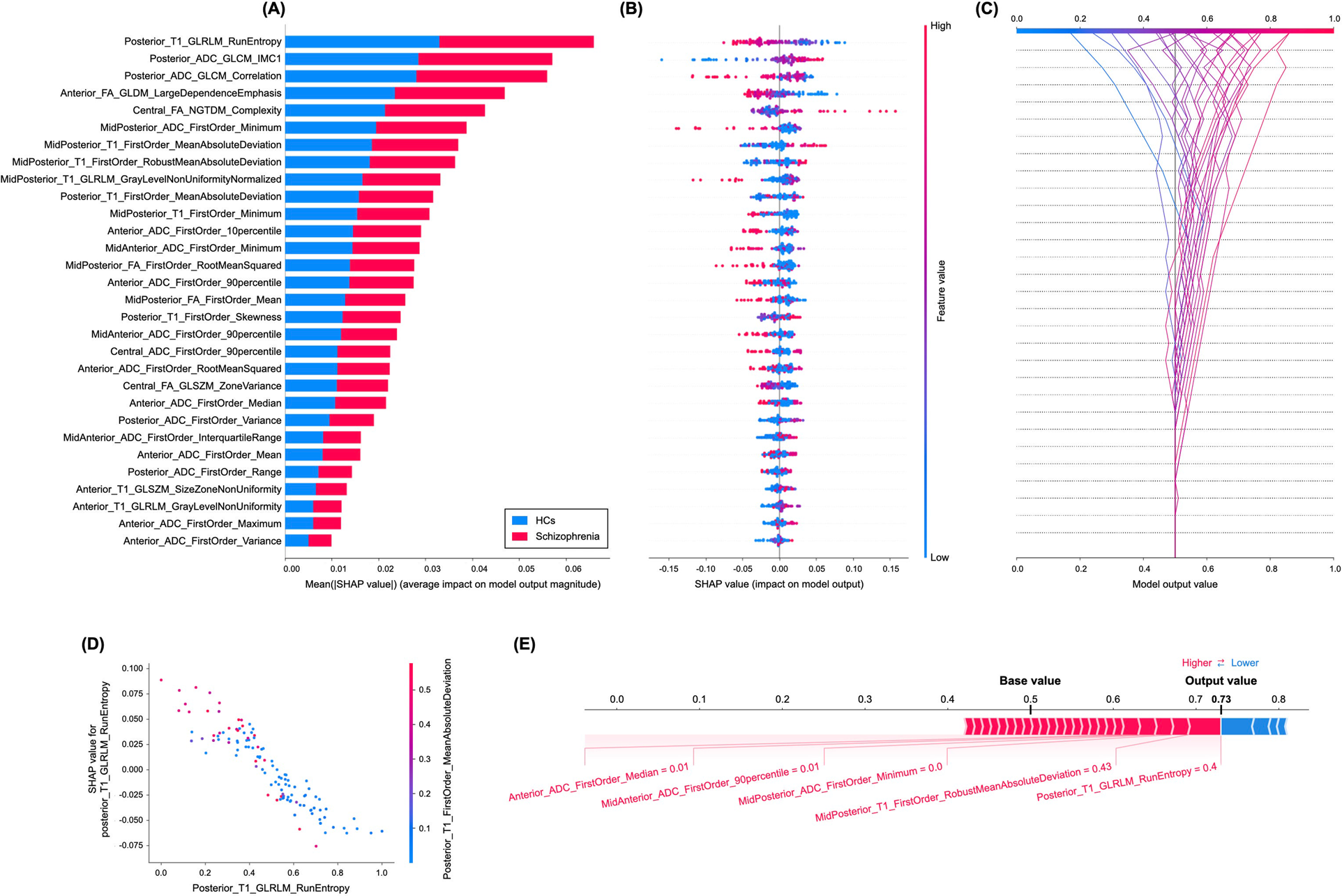
Figure 1. “A Variance importance plot listing the most significant variables in descending order. The top variables (such as posterior_T1_GLRLM_run entropy, posterior_ADC_GLCM_IMC1, and posterior_ADC_GLCM_correlation features) contribute more to the model than the bottom ones and thus have higher predictive power. B Summary plot of feature impact on the decision of the radiomics model and interaction between radiomics features in the model. A positive SHAP value indicates an increase in the risk of predicting schizophrenia and vice versa. The high value corresponds to a higher risk of schizophrenia. Each point corresponds to a prediction in each participant. C Decision plot showing how the radiomics model predicts schizophrenia. Moving from the bottom of the plot to the top, SHAP values for each feature are added to the model’s base value showing how each feature contributes to the overall prediction of schizophrenia. D An example of the dependence plot of the posterior_T1_GLRLM_run entropy feature, which is the top-most important feature. The plot shows how there is an approximately linear and negative trend between “posterior_T1_GLRLM_RunEntropy” and schizophrenia prediction, and that the “posterior_T1_GLRLM_RunEntropy” interacts with “posterior_T1_FirstOrder_MeanAbsoluteDeviation” frequently. E Force plot of a representative case of participants with schizophrenia from the test set, showing local interpretability. Note that the posterior_T1_GLRLM_RunEntropy largely pushes the model prediction score into the higher direction from the base value.” [2] (from the article by Bang et al.; licensed under CC BY 4.0)
Example#2. See Figure 2.
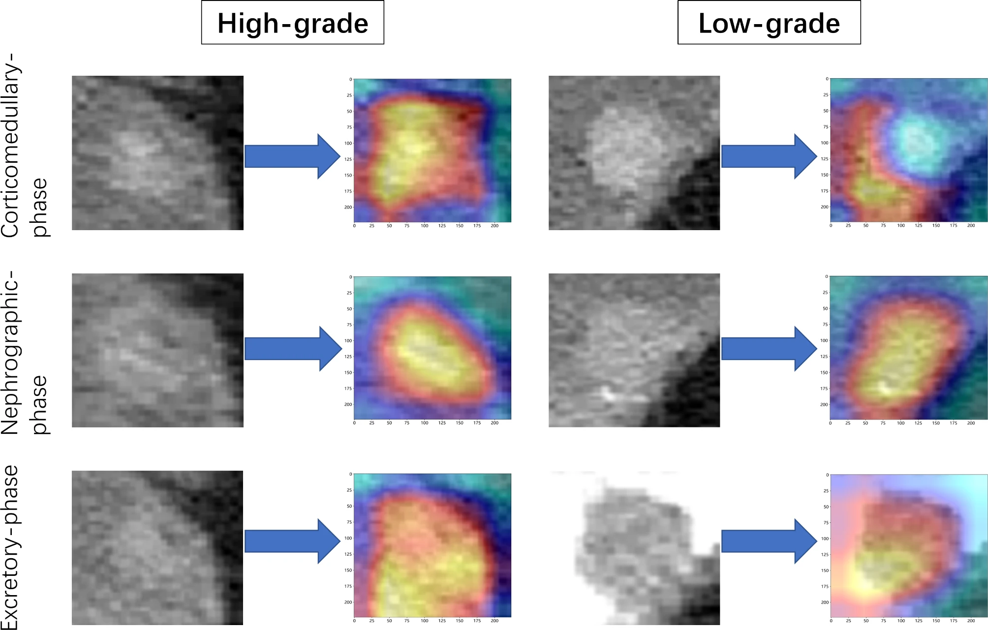
Figure 2. “Activation maps of the deep convolutional neural networks for high versus low grade bladder cancer, reflected the weights corresponding to different pathological grades of tumors. These maps were constructed using data from the corticomedullary phase, nephrographic phase, and excretory phase. Red areas indicate higher correlation with tumor grade” [3] (from the article by Song et al; licensed under CC BY 4.0)
Example#3. See Figure 3.
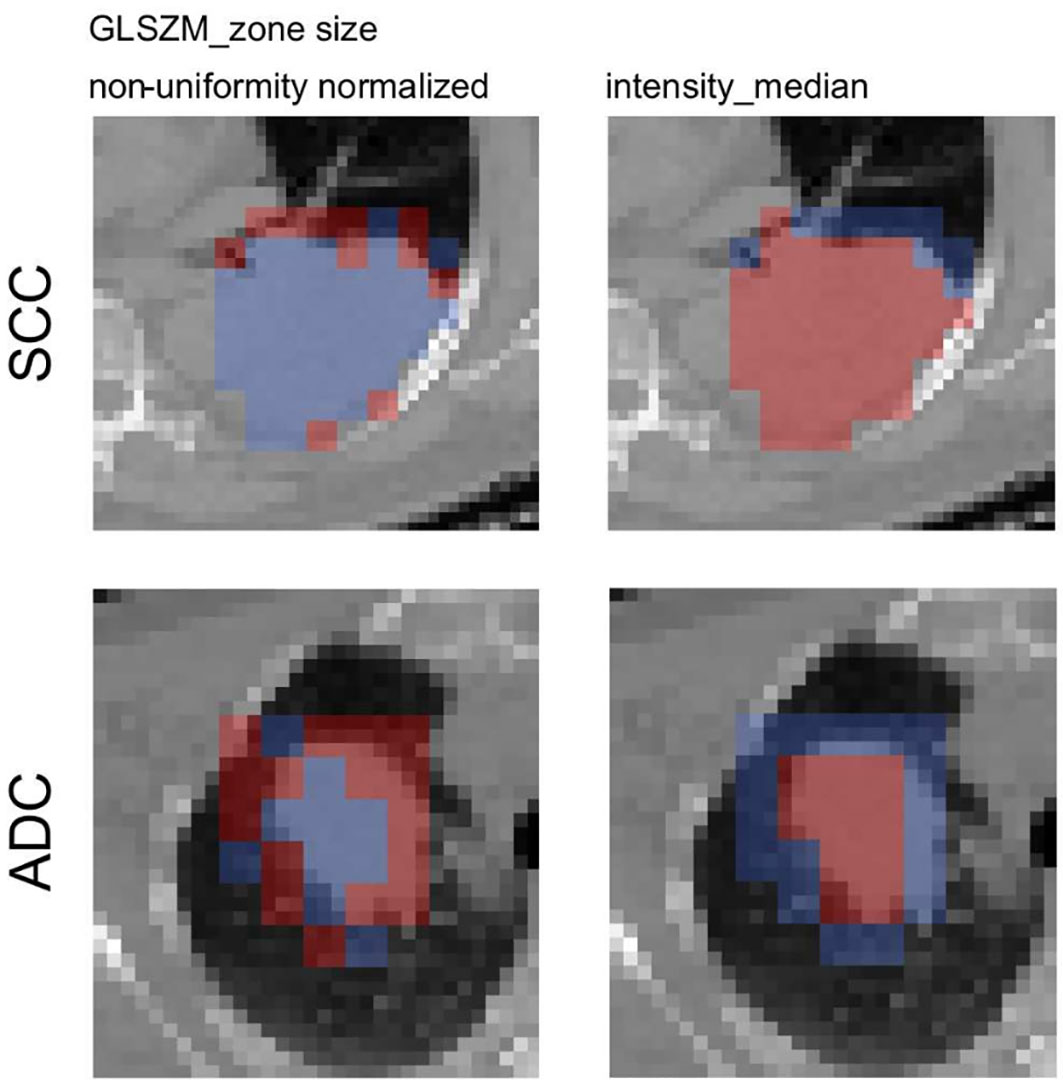
Figure 3. “Axial slices of the feature activation maps overlaid with the corresponding CT scan of a squamous cell carcinoma patient (SCC) and an adenocarcioma patient (ADC) from the validation cohort. Activated (red) patches had feature values larger than the median feature value from the training, whereas non-activated (blue) patches had feature values smaller than the median. The texture feature was activated mostly in the rim region whereas the intensity_median was activated mostly in the tumor region.” [4] (from the article by Vuong et al.; licensed under CC BY 4.0)
Explanation and elaboration of CLEAR item#43
The significance of providing interpretability and explainability methods in radiomics studies is emphasized in item#43. Clinicians are hesitant to adopt radiomics models due to the unclear internal mechanisms or unexplained features, with consequent lack of interpretability of radiomic models. Therefore, authors need to ensure that the results of their radiomics study may be explained based on reference standard and can be interpreted by the reader for clinical transferability. There are several methods for explainability and interpretability. Example#1 uses a SHapley Additive exPlanations method to illustrate the importance of the radiomics features and their impact on the overall prediction model and to understand the importance of individual features on the model output explanation. Example#2 benefits from a class activation map for deep learning-based approaches. Example#3 uses radiomics activation maps to track the spatial location of regions responsible for radiomic signature activation.
References
- Kocak B, Baessler B, Bakas S, et al (2023) CheckList for EvaluAtion of Radiomics research (CLEAR): a step-by-step reporting guideline for authors and reviewers endorsed by ESR and EuSoMII. Insights Imaging 14:75. https://doi.org/10.1186/s13244-023-01415-8
- Bang M, Eom J, An C, et al (2021) An interpretable multiparametric radiomics model for the diagnosis of schizophrenia using magnetic resonance imaging of the corpus callosum. Transl Psychiatry 11:1–8. https://doi.org/10.1038/s41398-021-01586-2
- Song H, Yang S, Yu B, et al (2023) CT-based deep learning radiomics nomogram for the prediction of pathological grade in bladder cancer: a multicenter study. Cancer Imaging 23:89. https://doi.org/10.1186/s40644-023-00609-z
- Vuong D, Tanadini-Lang S, Wu Z, et al (2020) Radiomics Feature Activation Maps as a New Tool for Signature Interpretability. Front Oncol 10. https://doi.org/10.3389/fonc.2020.578895