Condition #4
“Does the study include tabular data?” [1] (licensed under CC BY)
Explanation
“Tabular data refers to data that is organized in a table with rows and columns.” [1] (licensed under CC BY)
Examples from the literature meeting “Yes” condition
Example #1: “From each segmented lesion, 6,048 radiomic features were extracted representing shape, first-order, gray level co-occurrence matrix−GLCM, gray level run length matrix−GLRLM, gray level size zone matrix−GLSZM, gray level dependence matrix−GLDM, and neighboring gray tone difference matrix−NGTD features at three different levels of granularity (coarse, medium, and fine resampling). Feature extraction was performed using the open-source package pyradiomics v3.0 in compliance with Image Biomarker Standardization Initiative−IBSI standards. […]
The development of the MSI radiomic predictive signature involved a two-step feature reduction and selection process. Firstly, we used statistical testing to drop features influenced by segmentation and center-level differences. To account for center-level differences, we used the Kruskal-Wallis test to identify features significantly associated with the center of origin. Subsequently, to assess radiomic feature reproducibility due to inter-reader variability, we sampled 36 cases from the training set, and all three radiologists (N.B., F.C., and F.L.) performed segmentations. Features significantly affected by segmentation-level differences, as determined by Mann-Whitney U tests, were excluded from the analysis. Benjamini-Hochberg corrections were applied to adjust the significance levels for multiple testing and reduce the false discovery rate. The features deemed robust for center and segmentation were then taken to the second step comprising supervised feature selection using the MSI status outcome.
We used a supervised ensemble feature selection approach where, on the training set, six supervised feature selection techniques (namely, recursive feature extraction, Pearson correlation, χ2, logistic regression, light gradient boosting machine, and random forest) were independently tasked with selecting the top 100 features associated with the outcome on the training set. Radiomic features that achieved consensus on relevance (i.e., selection by four of six techniques) formed the radiomic signature. Ensemble feature selection methods have been shown to outperform single feature selection methods, generate more stable signatures, and scale to high dimensional data, including radiomics. Crucially, this selection step was performed solely on the internal training set, and external validation sets were never used in the second step of the feature selection process (where the MSI status was an input). Additionally, a correlation analysis was performed to ensure that the features in the radiomic signature were sufficiently independent.” [2] (licensed under CC BY)
Example #2: “Features extraction and features selection We used a feature analysis program designed for radiomics analysis within Pyradiomics to extract radiomic features. The extracted features were classified into three primary categories: geometry, intensity, and texture. The geometry feature depicts the shape characteristic of the lesion. The intensity feature illustrates the first-order statistical distribution of voxel intensity within the lesion. Texture features describe the pattern or the second- and high-order spatial distribution of the intensity, including gray-level co-occurrence matrix (GLCM), gray-level dependence matrix, gray-level size zone matrix, gray-level run-length matrix, and neighboring gray-tone difference matrix.
To identify features that exhibited the strongest correlation with the categorization, we employed the t-test and the Mann–Whitney U-test to screen features. We retained features associated with a p value less than 0.05, as they indicated significant differences between the two sets. To eliminate superfluous features, the correlation among the features was ascertained by calculating Spearman’s rank correlation coefficient. We selected only one feature from any pair presenting a correlation coefficient exceeding 0.9 to remove those exhibiting high redundancy. Additionally, we adopted a greedy recursive deletion approach to filter features, which involves the iterative removal of features deemed most superfluous in the current set.
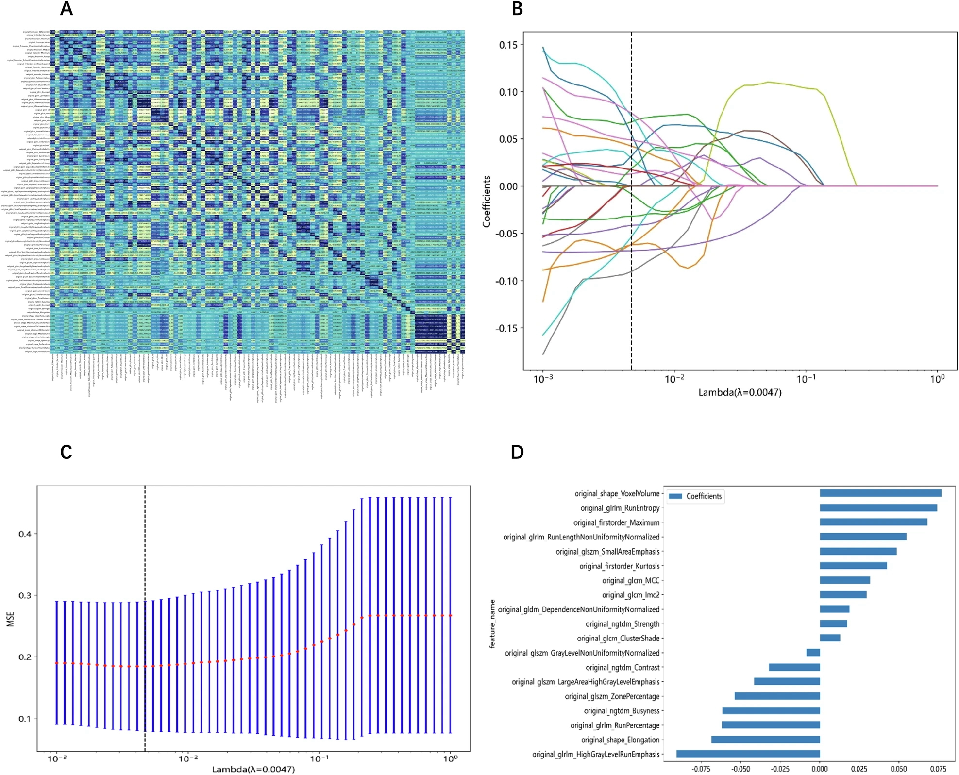
We utilized the least absolute shrinkage and selection operator (LASSO) regression to minimize the feature set. The Rad scores were generated using LASSO logistic regression (LR), selecting only the features with non-zero coefficients. LASSO shrank all regression coefficients towards 0, depending on the regulation weight λ, and precisely set the coefficient of the uncorrelated feature to 0. The optimal λ value was ascertained through 10-fold cross-validation using minimum criteria, and the ultimate λ induced the least cross-validation error. The most robust feature with a non-zero coefficient was utilized for regression model fitting and integrated into a radiomic signature. A Rad score was generated from a linear combination of the selected features, each weighted according to the corresponding model coefficient.
Model construction and evaluation
We utilized Python to establish radiomic and clinical models. The selected features were put into several machine learning algorithms, including LR, support vector machine (SVM), k-nearest neighbor (KNN), Random Forest, XGBoost, LightGBM, and multi-layer perception (MLP). We subsequently conducted a 5-fold cross-validation to ascertain the best hyperparameters for model fitting. A radiomic nomogram was developed, incorporating both radiomic features and clinical features for analysis.” [3] (licensed under CC BY)
Also see Figure 1.
Figure 1. “Feature extraction and selection. A Spearman correlation coefficient between each feature. B Coefficients of 10-fold cross-validation based on LASSO algorithm. C MSE of 10-fold cross-validation based on LASSO algorithm. D Histogram depicting the values of coefficients in the final selected non-zero features. MSE, mean square error” [3] (licensed under CC BY)
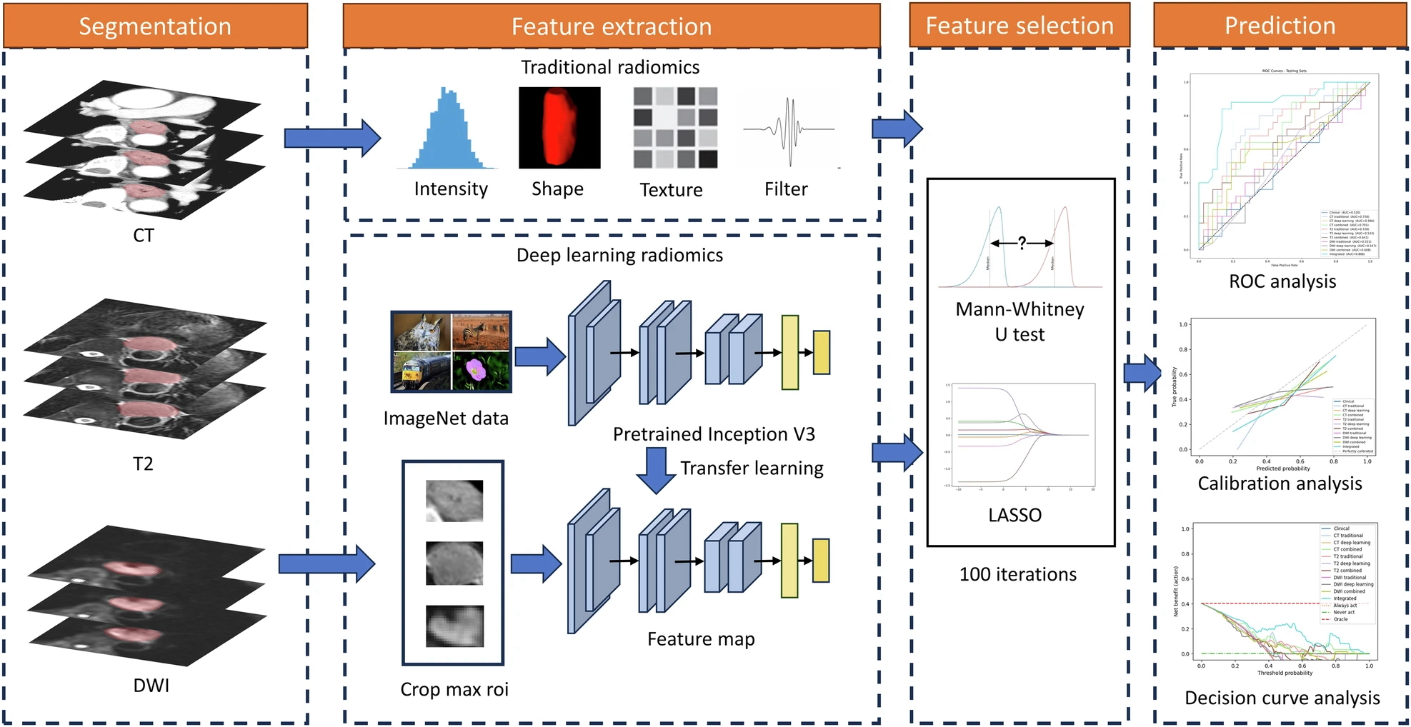
Example #3: “Z-score normalization was implemented before extracting traditional features. A total of 1652 features were extracted from both original and filtered images. For deep learning, the Inception-V3 network, pre-trained on ImageNet data, was employed. The largest tumor images from each patient were cropped for feature extraction, with grayscale values normalized within the range [−1, 1] using min–max transformation. The images were then resized to 299 × 299 using the nearest interpolation. The network’s last fully connected layer was removed, and the average pooling layer of the feature maps was used to extract 2048 deep-learning features.” [4] (licensed under CC BY)
Also see Figure 2.
Figure 2. “Workflow of the radiomics analysis” [4] (licensed under CC BY)
Hypothetical examples meeting “No” condition
Example #4: A convolutional neural network (CNN) was developed for automated tumor classification using contrast-enhanced CT images. The model consisted of five convolutional layers, each followed by batch normalization and max-pooling. The final feature maps were flattened and passed through two fully connected layers before classification into benign or malignant tumors. The model was trained using categorical cross-entropy loss and evaluated using accuracy, precision, and recall metrics.
Example #5: We developed a self-supervised learning approach for tumor segmentation. The model was trained on a dataset of 3,000 MRI scans without manual annotations. The model utilized contrastive embeddings learned through a Siamese neural network. These embeddings were used to cluster images based on their feature similarities, and the performance was evaluated using the Dice similarity coefficient (DSC) and Jaccard index.
Importance of the condition
This condition determines how radiomics feature data is processed, directly impacting which METRICS items need to be considered. Traditional radiomics features are typically treated as tabular data. Additionally, deep learning can also generate tabular data through feature extraction [5]. Any layer in such approaches can produce deep features, which resemble traditional radiomics features in format. These deep features are often processed similarly, using conventional radiomics analysis and machine learning algorithms.
Specifics about the examples meeting “Yes” condition
Example #1 clearly demonstrates traditional radiomics feature extraction and handling, where the resulting data is structured in a tabular format, as indicated in the provided text. Example #2 reinforces this concept, offering additional details on traditional machine learning models, which further support the identification of tabular data. Additionally, the accompanying figure highlights traditional feature names within the graphs, providing a visual cue to assess this condition more easily. Example #3 goes beyond traditional radiomics by incorporating deep feature extraction alongside conventional features, effectively illustrating both approaches in practice as a source for tabular data. The accompanying illustration (i.e., Figure 2) is also helpful in confirming that deep features are treated in a tabular format similar to conventional ones, as they undergo feature selection algorithms.
Specifics about the examples meeting “No” condition
In Example #4, a standard end-to-end CNN classifies tumors without extracting structured radiomic or deep-learning features in tabular form, as it learns features automatically. In Example #5, a self-supervised learning method generates image embeddings instead of using traditional radiomic features, requiring no tabular data processing, making it ineligible for the condition.
Recommendations for appropriate scoring
All traditional radiomics features should be classified as tabular data, making the condition easily classifiable as “Yes”.
However, caution is needed when evaluating deep features, as not all deep learning studies extract them in a structured format. Some deep learning models operate in an end-to-end manner, where features are inherently learned within the model rather than being explicitly extracted for separate handling. In such cases, manual feature extraction is not required, and the condition should be classified as “No”.
Therefore, when scoring, it is essential to distinguish between studies that explicitly extract deep features in tabular form (classified as “Yes”) and those that use end-to-end deep learning without feature extraction (classified as “No”).
References
- Kocak B, Akinci D’Antonoli T, Mercaldo N, et al (2024) METhodological RadiomICs Score (METRICS): a quality scoring tool for radiomics research endorsed by EuSoMII. Insights Imaging 15:8. https://doi.org/10.1186/s13244-023-01572-w
- Bodalal Z, Hong EK, Trebeschi S, et al (2024) Non-invasive CT radiomic biomarkers predict microsatellite stability status in colorectal cancer: a multicenter validation study. European Radiology Experimental 8:98. https://doi.org/10.1186/s41747-024-00484-8
- Liu L, Cai W, Zheng F, et al (2025) Automatic segmentation model and machine learning model grounded in ultrasound radiomics for distinguishing between low malignant risk and intermediate-high malignant risk of adnexal masses. Insights into Imaging 16:14. https://doi.org/10.1186/s13244-024-01874-7
- Liu Y, Wang Y, Hu X, et al (2024) Multimodality deep learning radiomics predicts pathological response after neoadjuvant chemoradiotherapy for esophageal squamous cell carcinoma. Insights into Imaging 15:277. https://doi.org/10.1186/s13244-024-01851-0
- Demircioğlu A (2023) Are deep models in radiomics performing better than generic models? A systematic review. Eur Radiol Exp 7:11. https://doi.org/10.1186/s41747-023-00325-0