Item #20
“Use of appropriate performance evaluation metrics for task” [1] (licensed under CC BY)
Explanation
“Whether appropriate accuracy metrics are reported, such as AUC for Receiver Operating Characteristics (ROC) or Precision-Recall (PRC) curves and confusion matrix-derived accuracy metrics (e.g., specificity, sensitivity, precision, F1 score) for classification tasks; MSE, RMSE, and MAE for regression tasks. For classification tasks, the confusion matrix should always be included, to allow the calculation of additional metrics. If training a DL network, loss curves should be presented.” [1] (licensed under CC BY)
Positive examples from the literature
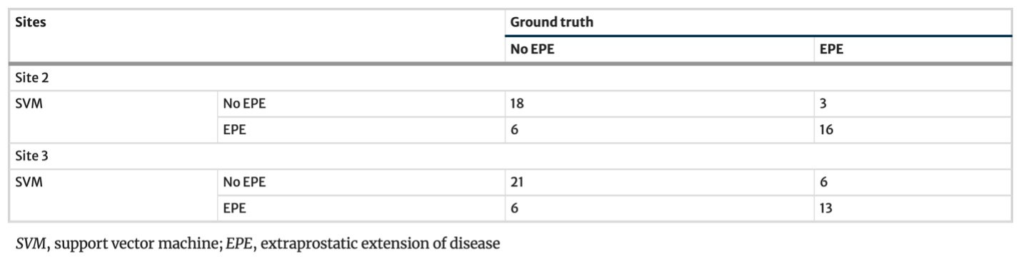
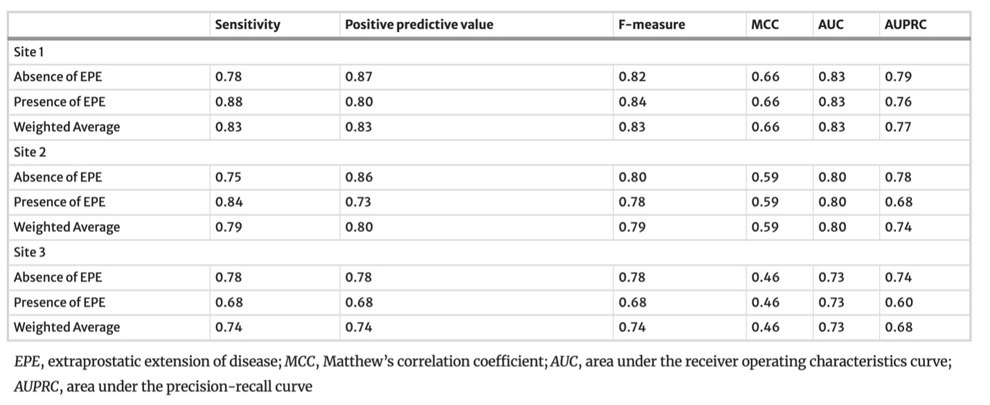
Example #1: “Confusion matrices and complete accuracy metrics are reported in [Table 1 and Table 2], respectively.” [2] (licensed under CC BY)
Table 1. “Confusion matrices for the SVM model” [2] (licensed under CC BY)
Table 2. “Accuracy metrics for the SVM model for the training (site 1) and testing (site 2 and site 3) datasets” [2] (licensed under CC BY)
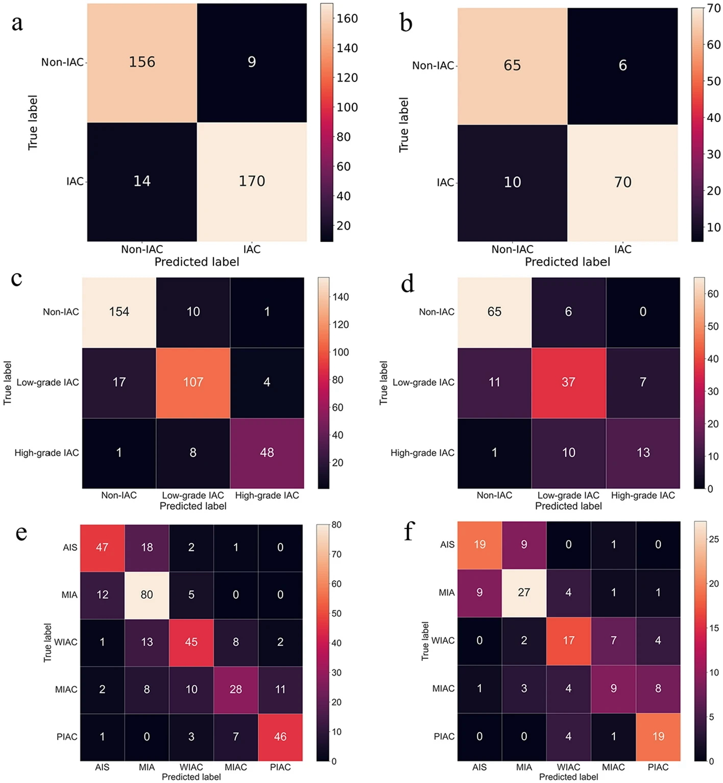
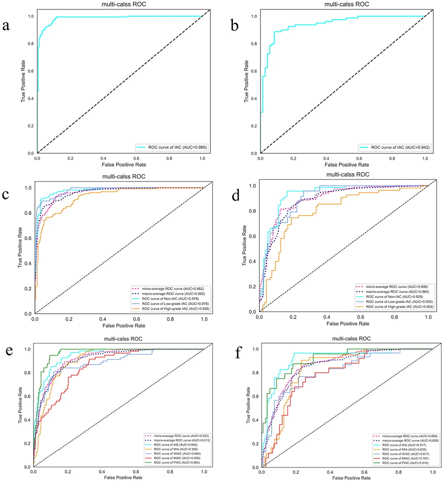
Example #2. “[Figure 1] displays the confusion matrix of the combined model using SVM and SVM-OVO in both the training and testing cohorts. The matrix illustrates that the selected models were not prone to making errors and effectively captured the relationships among histological subtypes. The ACC in the testing cohort exceeded 0.6, even for the challenging five-classification task. All histological subtypes in the three and five-classification tasks were accurately identified. The macro-AUC and micro-AUC values of the three-classification model in the testing cohort were 0.884 and 0.896, respectively. Similarly, the macro-AUC and micro-AUC values of the five-classification model were 0.858 and 0.866, respectively. The AUC values of the histological subtypes ranged from 0.787 to 0.942, with the lowest AUC observed for MIAC in the testing cohort, as depicted in [Figure 2]” [3] (licensed under CC BY).
Figure 1. “Confusion matrix on radiomics combined model: the two-classification in train cohort (a) and test cohort (b), the three-classification in train cohort (c) and test cohort (d), and the five-classification in train cohort (e) and test cohort (f)” [3] (licensed under CC BY)
Figure 2. “ROC curve on radiomics combined model: the two-classification in train cohort (a) and test cohort (b), the three-classification in train cohort (c) and test cohort (d), and the five-classification in train cohort (e) and test cohort (f)” [3] (licensed under CC BY)
Example #3. “We observed that the performance on the internal data strongly varied across the different ML models: when using all features, r ranged from 0.44 for the LR model to 0.73 for the RFR model, and MAE varied from a maximum of 138.0 for the LR model to a minimum of 13.9 for the RFR model” [4] (licensed under CC BY)
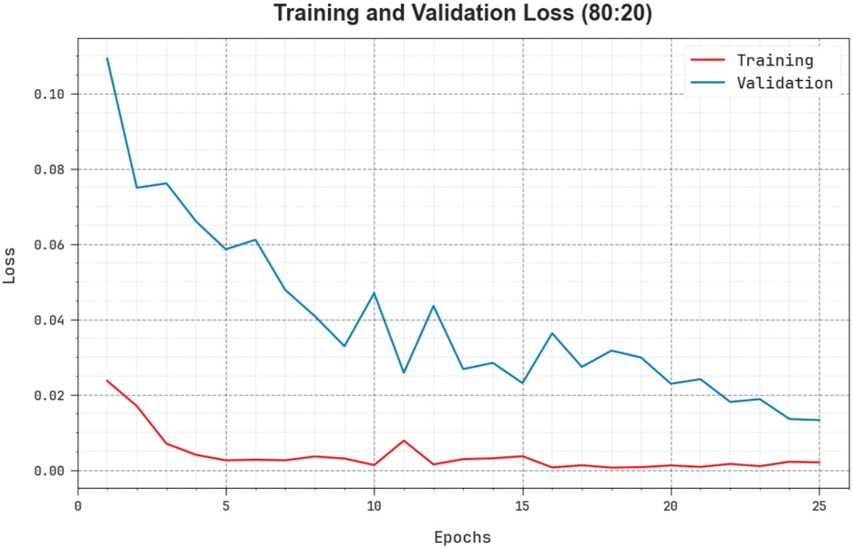
Example #4. “The comprehensive TR and TS loss values of the EOADL-PCDC system on 80:20 of TRAP/TESP over epochs are shown in [Figure 3]. The TR loss states the model loss minimized over epochs. Initially, the loss value is minimized as the model adapts the weight to minimize the predictive error on the TR and TS datasets. The loss curve exhibits the level where the model fits the training dataset. The TR and TS loss reduced progressively and showed that the EOADL-PCDC method efficiently learns the patterns given in the TR and TS datasets” [5] (licensed under CC BY)
Figure 3. “Loss curve of the EOADL-PCDC system on 80:20 of TRAP/TESP.” [5] (licensed under CC BY)
Hypothetical negative examples
Example #5: We developed a radiomic model to classify breast lesions on mammograms as either benign or malignant. Our dataset consisted of 1000 mammograms, with 600 labeled as benign and 400 as malignant. We obtained a precision of 85% (95% CI: 78% - 92%) and a recall of 75% (95% CI: 66% - 84%). The F1-score was 0.80. The area under the precision-recall curve (AUPRC) was 0.82. The model demonstrated good generalization performance on the test set.
Example #6: We developed a radiomics model to discriminate between Alzheimer’s Disease (AD) and Mild Cognitive Impairment (MCI) using structural MRI data. Our dataset comprised 300 individuals: 100 with AD, 100 with MCI, and 100 healthy controls. We focused on differentiating AD from MCI. The model was trained on a randomly selected 70% of the AD and MCI subjects (140 subjects total) and tested on the remaining 30% (60 subjects total). We employed a Support Vector Machine (SVM) classifier with a radial basis function kernel. Performance was evaluated using several metrics. The model achieved an Area Under the Receiver Operating Characteristic Curve (AUC) of 0.88 (95% CI: 0.80 - 0.96). Sensitivity, representing the ability to correctly identify AD patients, was 82% (95% CI: 70% - 94%). Specificity, representing the ability to correctly identify MCI patients, was 78% (95% CI: 65% - 91%).
Example #7: We trained a deep learning convolutional neural network (CNN) to segment lesions in brain MRI scans. The network architecture consisted of [details of the CNN architecture]. We used a dataset of 200 patients, splitting it into 80% for training and 20% for validation. [Figure X] shows the training and validation accuracy over 50 epochs. As seen, the accuracy improved steadily and reached a plateau, with a final validation accuracy of 92%, indicating good convergence. We also monitored the Dice coefficient during training, and the average Dice on the validation set was 0.88.
Example #8: We trained a deep learning convolutional neural network (CNN) to classify brain MRI scans as either glioblastoma or metastasis. The network architecture consisted of [details of the CNN architecture]. We used a dataset of 200 patients, splitting it into 80% for training and 20% for validation. The model achieved an area under the ROC curve (AUC) of 0.91 (95% CI: 0.85 - 0.97). Sensitivity was 85% (95% CI: 74% - 96%), and specificity was 88% (95% CI: 78% - 98%). [Table X] shows the confusion matrix. [Figure X] shows the training and validation accuracy curves over 50 epochs, demonstrating steady improvement and convergence at a validation accuracy of 90%.
Importance of the item
In radiomics studies, selecting the appropriate accuracy metrics is crucial for reliably evaluating model performance and clinical relevance. Given that radiomics-based models often analyze complex imaging data, accurate evaluation becomes essential [6]. Although the final applications may be complex, machine learning (ML) and deep learning (DL) models generally consist of simpler sub-tasks, such as binary or multi-class classification and regression. Depending on the specific task, different evaluation metrics can be employed to assess model performance effectively. Using appropriate accuracy metrics serves two key purposes: it allows for the elimination of underperforming methods and facilitates the optimization of promising models [7]. Moreover, utilizing suitable metrics enhances reproducibility, enabling reliable comparisons across studies and ensuring that these models are both robust and clinically useful [8]. A good general practice is represented by including the source data required to extrapolate the relevant accuracy metrics (e.g., confusion matrices for discrete accuracy metrics).
Specifics about the positive examples
Example #1 represents an excellent example, since the final model performance for detecting extraprostatic extension of disease was independently tested on 2 external datasets calculating confusion matrix-derived accuracy metrics and ROC curves. Like Example #1, the authors in Example #2 presented their confusion matrices for radiomics-based models, predicting the invasiveness and differentiation of pulmonary adenocarcinoma nodules, in a figure format instead of a table, achieving a positive score. When evaluating regression tasks, it is crucial to adopt specific accuracy metrics tailored to the context of the analysis. For instance, in Example #3, the authors correctly utilized the MAE to assess the difference between predicted and actual plasma cell infiltration either in internal or external datasets. Loss curves are essential in training DL models, as they provide valuable insights into learning progress, help detect overfitting or underfitting, and should always be presented, as demonstrated in Example #4.
Specifics about the negative examples
Example #5 lacks essential accuracy metrics like sensitivity and specificity, which are crucial for evaluating medical classification tasks comprehensively. It also has no confusion matrix, which may have allowed calculation of these metrics. Similarly, Example #6 does not present or mention a confusion matrix, preventing evaluation of classification accuracy beyond the reported metrics. Example #7 incorrectly relies solely on accuracy curves, which reflect model performance indirectly; it omits loss curves, even though loss curves directly represent the optimization objective guiding parameter adjustments (weights and biases). Without presenting loss curves, it is not possible to assess training stability, convergence, or detect potential issues like overfitting or underfitting in deep learning models. Example #8 also shows a slightly modified classification version of the Example #7, giving all classification metrics but the loss curve.
Recommendations for appropriate scoring
When evaluating the appropriate adoption of performance evaluation metrics in radiomics papers, it is essential to clearly identify the specific tasks the authors aimed to assess, which may include binary and multiclass classification, regression, or image segmentation. For classification tasks, metrics such as AUC for ROC curves and PRC curves should have been utilized, as well as MSE or MAE for regression tasks. For classification, sensitivity and specificity should always be reported because these are essential metrics in medical context.
To receive the item score for the classification tasks, it is mandatory that the authors have reported a confusion matrix.
In addition to the above metrics that are appropriate for the task of interest, a positive rating should not be given to papers that trained DL algorithms but did not present the loss curves to monitor learning progress.
References
- Kocak B, Akinci D’Antonoli T, Mercaldo N, et al (2024) METhodological RadiomICs Score (METRICS): a quality scoring tool for radiomics research endorsed by EuSoMII. Insights Imaging 15:8. https://doi.org/10.1186/s13244-023-01572-w
- Cuocolo R, Stanzione A, Faletti R, et al (2021) MRI index lesion radiomics and machine learning for detection of extraprostatic extension of disease: a multicenter study. Eur Radiol 31:7575–7583. https://doi.org/10.1007/s00330-021-07856-3
- Sun H, Zhang C, Ouyang A, et al (2023) Multi-classification model incorporating radiomics and clinic-radiological features for predicting invasiveness and differentiation of pulmonary adenocarcinoma nodules. BioMed Eng OnLine 22:112. https://doi.org/10.1186/s12938-023-01180-1
- Wennmann M, Rotkopf LT, Bauer F, et al (2025) REPRODUCIBLE RADIOMICS FEATURES FROM MULTI‐MRI‐SCANNER TEST–RETEST‐STUDY: INFLUENCE ON PERFORMANCE AND GENERALIZABILITY OF MODELS. Magnetic Resonance Imaging 61:676–686. https://doi.org/10.1002/jmri.29442
- Yang E, Shankar K, Kumar S, et al (2023) Equilibrium Optimization Algorithm with Deep Learning Enabled Prostate Cancer Detection on MRI Images. Biomedicines 11:3200. https://doi.org/10.3390/biomedicines11123200
- Lambin P, Leijenaar RTH, Deist TM, et al (2017) Radiomics: the bridge between medical imaging and personalized medicine. Nat Rev Clin Oncol 14:749–762. https://doi.org/10.1038/nrclinonc.2017.141
- Rainio O, Teuho J, Klén R (2024) Evaluation metrics and statistical tests for machine learning. Sci Rep 14:6086. https://doi.org/10.1038/s41598-024-56706-x
- Hicks SA, Strümke I, Thambawita V, et al (2022) On evaluation metrics for medical applications of artificial intelligence. Sci Rep 12:5979. https://doi.org/10.1038/s41598-022-09954-8